5.1.3 Display and Initial Analysis

As described in the previous subsection, hackcode1 writes various diagnostics in the output file. A summary of conservation of energy and center-of-mass motion can be graphically displayed using snapdiagplot:

    10% snapdiagplot in=r001.dat

The program snapplot displays the evolution of the particle distribution, in projection;

    11% snapplot in=r001.dat

Depending on the actual graphics (yapp) interface of snapplot, you may have to hit the RETURN key, push a MOUSE BUTTON or just WAIT to advance from one to the next frame.

The snapplot program has a very powerful tool built into it which makes it possible to display any ``projection'' the user wants.

As an example consider:

    12% snapplot in=r001.dat xvar=r yvar="x*vy-y*vx" xrange=0:10 \
               yrange=-2:2 "visib=-0.2<z&&z<0.2&&i%2==0"

plots the angular momentum of the particles along the z axis, $J_z = x*v_y - y*v_x$, against their radius, $r$, but only for the even numbered particles, (i%2==0) within a distance of 0.2 of the X-Y plane ($-0.2<z \&\& z<0.2$). Again note that some of the expressions are within quotes, to prevent the shell of giving them a special meaning.

The xvar, yvar and visib expressions are fed to the C compiler (during runtime!) and the resulting object file is then dynamically loaded into the program for execution^5.5. The expressions must contain legal C expressions and depending on their nature must return a value in the context of the program. E.g. xvar and yvar must return a real value, whereas visib must return a boolean (false/true or 0/non-0) value. This should be explained in the manual page of the corresponding programs.

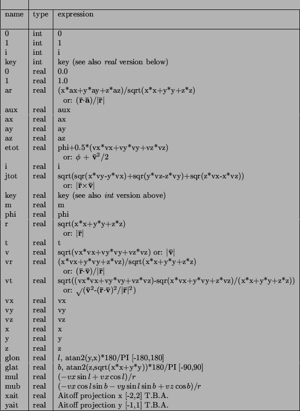
In the context of snapshots, the expression can contain basic body variables which are understood to the bodytrans(3NEMO) routine. The real variables x, y, z, vx, vy, vz are the cartesian phase-space coordinates, t the time, m the mass, phi the potential, ax,ay,az the cartesian acceleration and aux some auxiliary information. The integer variables are i, the index of the particle in the snapshot (0 being the first one in the usual C tradition) and key, another spare slot.

For convenience a number of expressions have already been pre-compiled (see also Table ), e.g. the radius r=$\sqrt{x^2+y^2+z^2}$=sqrt(x*x+y*y+z*z), and velocity v=$\sqrt{v_x^2+v_y^2+v_z^2}$=sqrt(vx*vx+vy*vy+vz*vz). Note that r and v themselves cannot be used in expressions, only the basic body variables listed above can be used in an expression.

When you need a complex expression that has be used over and over again, it is handy to be able to store these expression under an alias for later retrieval. With the program bodytrans it is possible to save such compiled expressions object files under a new name.

Table: Some precompiled bodytrans expressions

As usual an example:

    13% bodytrans expr="x*vy-y*vz" type=real file=jz

saves the expression for the angular momentum in a real valued bodytrans expression file, btr_jz.o which can in future programs be referenced as expr=jz (whenever a real-valued bodytrans expression is required), e.g.

    14% snapplot i001.dat xvar=r yvar=jz xrange=0:5

Alternatively, one can handcode a bodytrans function, compile it, and reference it locally. This is useful when you have truly complicated expressions that do not easily write themselves down on the commandline. The $(x,y)$ AITOFF projection are an example of this. For example, consider the following code in a (local working directory) file btr_r2.c:

    #include <bodytrans.h>

    real btr_r2(b,t,i)
    Body *b;
    real t;
    int  i;
    {
        return sqrt(x*x + y*y);
    }

By compiling this:

    15% cc -c btr_r2.c

an object file btr_r2.o is created in the local directory, which could be used in any real-valued bodytrans expression:

    16% snapplot i001.dat xvar=r2 yvar=jz xrange=0:5

For this your environment variable BTRPATH must have been set to include the local working directory, designated by a dot. Normally your NEMO system manager will have set the search path such that the local working directory is searched before the system one (in $NEMOOBJ/bodytrans).