5. Examples
Now that we have a reasonable idea how NEMO is structured and used, we
should be ready to go through some real examples Some of the examples
below are short versions of scripts available online in one of the
directories (check $NEMO/scripts and $NEMOBIN). The manual
pages programs(8NEMO) and intro(1NEMO) are useful to find (and
cross-reference) programs if you’re a bit lost. Each program manual
should also have some references to closely related programs,
in the “SEE ALSO” section.
5.1. N-body experiments
In this section we will describe how to set up an N-body experiment, run, display and analyze it. In the first example, we shall set up a head-on collision between two spherical “galaxies” and do some simple analysis.
5.1.1. Setting it up
In Filestructure we already used mkplummer to create a Plummer model;
so here we shall use the program mkommod
(“MaKe an Osipkov-Merritt MODel”)
to make two random N-body realizations of a King model
with dimensionless central potential \(W_c = 7\) and 100 particles each.
The small number of particles is solely for the purpose of getting
results within a reasonable time. Adjust it to whatever you can afford
on your CPU and test your patience and integrator.
1% mkommod in=$NEMODAT/k7isot.dat out=tmp1 nbody=100 seed=123
These models are produced in so-called RMS-units in which the
gravitational constant \(G=1\), the total mass \(M=1\), and binding energy
\(E=-1/2\).
In case you would like virial units (also known as N-body units)
(see also:
Heggie & Mathieu, \(E=-1/4\),
in: The use of supercomputers in stellar
dynamics ed. Hut & McMillan
Springer 1987, pp.233)
the models have
to be rescaled using snapscale:
2% snapscale in=tmp1 out=tmp1s rscale=2 "vscale=1/sqrt(2.0)"
Note the use of the quotes in the expression, to prevent the shell to give special meaning to the parenthesis, which are shell meta characters.
The second galaxy is made in a similar way, with a different seed (the default seed=0 takes the time of the day):
3% mkommod in=$NEMODAT/k7isot.dat out=tmp2 nbody=100 seed=987
This second galaxy needs to be rescaled too, if you want virial units:
4% snapscale in=tmp2 out=tmp2s rscale=2 "vscale=1/sqrt(2.0)"
We then set up the collision by stacking the two snapshots, albeit with
a relative displacement in phase space. The program snapstack was exactly
written for this purpose:
5% snapstack in1=tmp1s in2=tmp2s out=i001.dat deltar=4,0,0 deltav=-1,0,0
The galaxies are initially separated by 4 unit length and approaching
each other with a velocity consistent with infall from infinity
(parabolic encounter). The particles assembled in the data file
i001.dat are now ready to be integrated.
To look at the initials conditions we could use:
6% snapplot i001.dat xrange=-5:5 yrange=-5:5
which is displayed in Figure X
5.1.2. Integration using hackcode1
We then run the collision for 20 time units, with the standard N-body integrator based on the Barnes “hierarchical tree” algorithm:
7% hackcode1 in=i001.dat out=r001.dat tstop=20 freqout=2 \
   freq=40 eps=0.05 tol=0.7 options=mass,phase,phi > r001.log
The integration frequency relates to the integration timestep as
freq=40, the softening length eps=0.05, and
opening angle or tolerance tol=theta. A major output of
masses, positions and potentials of all particles is done every
1/freqout = 0.5 time units, which corresponds to about 1/5 of a
crossing time. The standard output of the calculation is diverted to a
file r001.log for convenience. This is an (ASCII) listing,
containing useful statistics of the run, such as the efficiency of the
force calculation, conserved quantities etc. Some of this information
is also stored in diagnostic sets in the structured binary
output file r001.dat.
As an exercise, compare the output of the following two commands:
8% more r001.log
9% tsf r001.dat | more
5.1.3. Display and Initial Analysis
As described in the previous subsection, hackcode1 writes various
diagnostics
in the output file. A summary of conservation of energy and center-of-mass
motion can be graphically displayed using snapdiagplot:
10% snapdiagplot in=r001.dat
The program snapplot displays the evolution of the particle
distribution, in projection (in the yt package this is called
a phase plot):
11% snapplot in=r001.dat
Depending on the actual graphics (yapp) interface snapplot was compiled with, you may have to hit the RETURN key, push a MOUSE BUTTON or just WAIT to advance from one to the next frame.
The snapplot program has a very powerful tool built into it
which makes it possible to display any projection the user wants.
As an example consider:
12% snapplot in=r001.dat xvar=r yvar="x*vy-y*vx" xrange=0:10 yrange=-2:2 \
             "visib=-0.2<z&z<0.2&i%2==0"
plots the angular momentum of the particles along the \(z\) axis,
\(J_z = x.v_y - y.v_x\) ,
against their radius, \(r\), but only for the even numbered particles,
(i%2==0) within
a distance of 0.2 of the X-Y plane (\(-0.2<z \& z<0.2\)).
Again note that some of the expressions are within quotes, to prevent
the shell of giving them a special meaning.
The xvar, yvar and visib expressions are fed to the
C compiler (during runtime!) and the resulting object file is then
dynamically loaded into the program for
execution.
The expressions must contain legal C expressions and depending
on their nature must return a value in the context of the
program. E.g. xvar and yvar must return a
real value, whereas visib must return a boolean (false/true or
0/non-0) value. This should be explained in the manual page of the
corresponding programs.
In the context of snapshots, the expression can contain
basic body variables which
are understood to the bodytrans(3NEMO) routine.
The real
variables x, y, z, vx, vy, vz are the cartesian phase-space
coordinates, t the time,
m the mass, phi the potential,
ax,ay,az the cartesian acceleration and aux
some auxiliary information.
The integer variables are
i, the index of the particle in the snapshot (0 being the
first one in the usual C tradition) and key, another
spare slot.
For convenience a number of expressions have already been pre-compiled
(see also Table ref{t:bodytrans}),
e.g. the radius r= \(\sqrt{x^2+y^2+z^2}\) = sqrt(x*x+y*y+z*z),
and velocity v = \(\sqrt{v_x^2+v_y^2+v_z^2}\) = sqrt(vx*vx+vy*vy+vz*vz). Note that r and
v themselves cannot be used in expressions, only the basic
body variables listed above can be used in an expression.
When you need a complex expression that has be used over and
over again, it is handy to be able to store these expression under
an alias for later retrieval.
With the program bodytrans
it is possible to save such compiled expressions object files under
a new name.
name |
type |
expression |
|---|---|---|
0 |
int |
|
1 |
int |
|
i |
int |
|
key |
int |
|
0 |
real |
|
1 |
real |
|
r |
real |
|
ar |
real |
|
at |
real |
|
aux |
real |
|
ax |
real |
|
ay |
real |
|
az |
real |
|
etot |
real |
|
i |
real |
|
jtot |
real |
|
key |
real |
|
m |
real |
|
phi |
real |
|
r |
real |
|
t |
real |
|
v |
real |
|
vr |
real |
|
vt |
real |
|
vx |
real |
|
vy |
real |
|
vz |
real |
|
x |
real |
|
y |
real |
|
z |
real |
|
glon |
real |
\(l\) , |
glat |
real |
\(b\) , |
mul |
real |
|
mub |
real |
\((-vx\cos{l}\sin{b} - vy\sin{l}\sin{b}+vz\cos{b})/r\) |
xait |
real |
Aitoff projection x [-2,2] T.B.A. |
yait |
real |
Aitoff projection y [-1,1] T.B.A. |
ra |
real |
Right Ascension, converted from radians to degrees (-x) |
dec |
real |
Declination, converted from radians to degrees (y) |
Here is an example of its use:
13% bodytrans expr="x*vy-y*vz" type=real file=jz
this saves the expression for the angular momentum in a real
valued bodytrans expression file, btr_jz.so which can in future programs
be referenced as expr=jz (whenever a real-valued bodytrans
expression is required), e.g.
14% snapplot i001.dat xvar=r yvar=jz xrange=0:5
Alternatively, one can handcode a bodytrans function, compile it,
and reference it locally. This is useful when you have truly complicated
expressions that do not easily write themselves down on the commandline.
The (x,y) AITOFF projection are an example of
this. For example, consider the following code in a (local working directory)
file btr_r2.c:
#include <bodytrans.h>

real btr_r2(b,t,i)
Body *b;
real t;
int  i;
{
    return sqrt(x*x + y*y);
}
By compiling this:
15% bake btr_r2.so
a shared object file btr_r2.so is created in the local directory,
which could be used in any real-valued bodytrans expression:
16% snapplot i001.dat xvar=r2 yvar=jz xrange=0:5
For this your environment variable BTRPATH
must have been set to include the local working directory,
designated by a dot. Normally your NEMO system manager will have set
the search path such that the local working directory is searched before
the system one (in $NEMOOBJ/bodytrans).
5.1.4. Advanced Analysis
more to come
5.1.5. Generating models
more to come
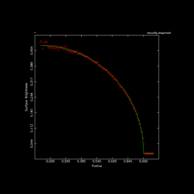
5.1.6. Using Unix pipes
In most cases a NEMO file can be used in a pipe (usually via
in=- and out=-), therefore limiting the need to write
files. Here is an example of plotting the measured and expected
surface brightness of a homogeneous sphere of 1,000,000 particles with
unit mass and unit radius:
1 % mkconfig - 1000000 ball seed=0 |\
2     snapgrid - - nx=800 ny=800  |\
3     ccdellint - 0:1.1:0.01 inc=0 out=- |\
4     ccdprint - x=  newline=t label=x |\
5     tabmath - - '1.5/pi*sqrt(1-%1**2)' |\
6     tabplot -  1 2,3 color=2,3 line=0,0,1,1 point=2,0.1,0,0 \
7       xlab="Radius" ylab="Surface Brightness" headline="mkconfig shape=ball" \
8       yapp=ball.png/png
A few comments on the highlighted lines: In line 3 the out= keyword is not the second keyword,
hence the explicit way it was written with the out=-.
In line 5 the expected surface brightness expression is added as the 3rd column to the table in the pipe,
then passed on for a quick and dirty plot (shown below).
5.1.7. Handling large datasets
One of NEMOs weaknesses is arguably also its strong point: programs must generally be able to fit all their data in (virtual) memory. Although programs usually free memory associated with data that is not needed anymore, there is a very clear maximum to the number of particles it can handle in a snapshot. By default a particle takes up about 100 bytes, which limits the size of a snapshots.
It may happen that your data was generated on a machine which had a lot more memory then the machine you want to analyze your data on. As long as you have the diskspace, and as long as you don’t need programs that cannot operate on data in serial mode, there is a solution to this problem. Instead of keeping all particles in one snapshot, they are stored in several snapshots of (equal number of) bodies, and as long as all snapshots have the same time and are stored back to back, most programs that can operate serially, will do this properly and know about it. Of course it’s best to split the snapshots on the machine with more memory
% snapsplit in=run1.out out=run1s.out nbody=10000
If it is just one particular program (e.g. snapgrid that needs a lot of extra memory, the following may work:
% snapsplit in=run1.out out=- nbody=1000 times=3.5 |\
    snapgrid in=- out=run1.ccd nx=1000 ny=1000 stack=t
Using tcppipe(1NEMO) one can also pipe data from the machine with large memory (A) to your workstation with smaller memory (B), as can be demonstrate with the following code snippet:
A% mkplummer - 1000 | tcppipe
B% tcppipe A | tsf -
5.2. Tables
Tables are obiquitous in astronomy in general and in NEMO specifically. Often they are simple ASCII tables, each row on a separate line and columns separated by a space or a comma (CSV). NEMO handles both, though generally output tables are space separated. NEMO’s table.5 man page goes in some more detail.
Intelligent tables (e.g. IPAC tables, the astropy ECSV format) add some header type information to annotate the table with column information (name, type, units) and sometimes even FITS-like provenance (e.g. IPAC tables). NEMO has limited ways to process these, currently loosing much of this header and provenance.
There is no good consistency in the programs if an out= keyword is needed, or if the table is written to stdout, or if out=- is the last parameter. Otherwise table programs are well suited for working the {tt pipe and filter} paradigm, as most NEMO programs are. Some examples are given below, with the caveat that the output pipe construction can be inconsistent.
Columns are typically given through the xcol= and ycol= keywords, and are 1-based. Column 0 has a special meaning, it is the row number (again 1 being the first row).
5.2.1. Manipulation
Here are some programs that manipulate tables:
tabgen was designed to produce tables from scratch, with some type of random values. Mostly to test performance and scalability of tables. Here a small table of 4 (rows) by 3 (columns) is written to *stdout:
% tabgen - nr=4 nc=3
0.552584 0.126911 0.520753
0.0930232 0.563683 0.258931
0.0369577 0.965763 0.634585
0.981766 0.334841 0.988963
tabcols selects columns from a table
tabrows selects rows from a table
tabtab takes two or more tables, and will paste (increasing the columns) or catenate (increasing the rows)
tabtranspose transposes the columns and rows of a table
% tabgen - nr=4 nc=3 | tabtranspose  - -
0.552584 0.0930232 0.0369577 0.981766
0.126911 0.563683 0.965763 0.334841
0.520753 0.258931 0.634585 0.988963
tabcomment comments out things that look like comments. Sometimes this filter is needed before another table program can be used, as they can get confused with non-numeric information. For example picking out two columns from a dirty table:
% tabcomment mytable.tab | tabcols - 2,3
...
tabcsv converts a table to some XSV, where X can be choosen from a set of characters
tabmath is a column calculator, but columns are referenced with a % sign, so %2 refers to column 2.. By default it will add the new columns to the old columns, unless some selection, or all, is/are removed. It can also select rows based on the values in a row, for example, only select rows where column 2 is positive.
Here is an example of adding two columns
% tabgen -  nr=4 nc=3 | tabmath - - %1+%2 all
0.679495
0.656706
1.00272
1.31661
txtpar extracts parameters from a text file. The often complex operations involving Unix tools such as grep/awk/sed/cut/head/tail can often be simplified with txtpar. Here is an example :
% cat example.txt
Worst fractional energy loss dE/E = (E_t-E_0)/E_0 = 0.00146761 at T = 1.28125
QAC_STATS: - 0.039966 0.0274195 0.00185505 0.135854  0.799319 1  20

% txtpar in=example.txt expr="log(abs(%1)),log(abs(%3/%2))" format=%.3f \
         p0=Worst,1,9  p1=QAC,1,3 p2=QAC,1,4
-2.833 -0.164
5.2.2. Generating
Some other NEMO programs that produce tables:
snapprint tabulates choosen body variables in ascii. The output format can also be choosen.
% mkplummer - 3 seed=123 | snapprint - comment=t format=%8.5f
#       x       y       z       vx      vy      vz
-2.19118 -0.01225  0.18687 -0.21951 -0.14248  0.28165
 3.22756 -0.27674 -0.88792  0.27564  0.18469  0.11529
-1.03638  0.28899  0.70105 -0.05613 -0.04221 -0.39694
5.2.3. Plotting
5.2.4. Analysis
tabtrend computes differences between successive rows
tabint integrate a sorted table
tabsmooth performs a smoothing operation on one or more columns
tablsqfit and tabnllsqfit do linear and non-linear fitting of functions
tabstat gives various statistics on selected columns
% tabgen - nr=4 nc=3 | tabstat - 1:3
npt:      4         4         4
min:      0.0369577 0.126911  0.258931
max:      0.981766  0.965763  0.988963
sum:      1.66433   1.9912    2.40323
mean:     0.416083  0.4978    0.600808
disp:     0.382993  0.311225  0.262247
skew:     0.424316  0.39325   0.250172
kurt:    -1.43956  -1.19861  -1.07587
min/sig: -0.989902 -1.19171  -1.30365
max/sig:  1.47701   1.50362   1.48011
median:   0.322804  0.449262  0.577669
5.3. Orbits
In this section we will describe how to integrate individual stellar orbits, display and analyze them. Be aware that although 3D orbits can be computed the number of utilities to analyze them is rather limited.
Orbits are normally stored in datafile (see also orbit(5NEMO)), and a close conceptual relationship exists between a (single-particle type) snapshot and an orbit: an orbit is an ordered series of phase-space coordinates whereas a snapshot is a series of particles with no particular order, but all at the same time.
Since orbits will be computed in an analytical potential, we assume for
the remainder of this section that you have familiarized yourself with
how to supply potentials to orbit integrator programs. They all share
the same triple potname=, potpars=, potfile= keyword
interface, as described in Section ref{s:potential}. Many
examples of the tricky potpars= keyword are given in Appendix
ref{a:potential}.
5.3.1. Initializing
There are a few programs with which orbits can be initialized:
mkorbit is the most straightforward program. You can give simply give it all 6 phase space coordinates, and an orbit file consisting of this one point is generated. It is also possible to give the potential in which the particle is to move, and 5 phase space coordinates plus the energy, or even 4 phase space coordinates and the energy plus the total angular momentum or angular momentum along the Z axis (for axisymmetric systems).
Let’s start with an example of creating a simple orbit by itself with no associated potential.
% mkorbit out=orb1 x=1 y=0 z=0 vx=0 vy=0.2 vz=0
### Warning [mkorbit]: Potential potname= not used; set etot=0.0
pos: 1.000000 0.000000 0.000000
vel: 0.000000 0.200000 0.000000
etot: 0.000000
lz=0.200000

% tsf orb1
char History[59] "mkorbit out=orb1 x=1 y=0 z=0 vx=0 vy=0.2 vz=0 VERSION=3.2b"
set Orbit
  set Parameters
    int Ndim 03
    double Mass 1.00000
    double IOM[3] 0.00000 0.200000 0.00000
    int Nsteps 01
  tes
  set Potential
  tes
  set Path
    double TimePath[1] 0.00000
    double PhasePath[1][2][3] 1.00000 0.00000 0.00000 0.00000 0.200000 0.00000
  tes
tes
perorb is a program that for given initial conditions (similar to the ones described in {tt mkorbit} above) attempts to calculate periodic orbits in that potential. The output file will be a file with one (or more) orbits. This is a bit of an advanced program, and will not be covered here.
stoo is a program that can take a particle position from a snapshot, and turn it into an orbit. For example, sampling some initial conditions from the positions of stars in a Plummer sphere, we could use the following small (bash) shell code to find some statistical properties of this selected set of orbitsfootnote{For the careful reader: mkplummer and potname=plummer actually have different units, and as such this experiment is not properly set up.}
mkplummer out=p100 nbody=p100
for i in $(nemoinp 0:100:10); do
    stoo in=p100 out=orb$i ibody=$i
    orbint orb$i orb$i.out 10000 0.01 10000 potname=plummer
    orbstat orb$i.out
done
The reverse program, otos turns an orbit into a snapshot, and may come in handy since the snapshot package has far more advanced analysis programs.
5.3.2. Integration
orbint integrates orbits from given initial conditions. If the input orbit has more than 1 step, the last step is taken as the initial conditions. Although the potname=, potpars=, potfile= keywords can be given, if the input orbit contains…
perorb finds periodic orbits, and stores a full period which should close the orbit. This program finds periodic orbits in the XY plane (i.e. currently it will only find 2D orbits) by searching for the centers of invariant curves in the surface of section.
henyey also finds periodic orbits, but uses Henyey’s methodfootnote{see also van Albada & Sanders, (1982, MNRAS, 201, 303)}. This program has however not been released to the public version of NEMO, and in fact it seems the source code was lost.
5.3.3. Display
orbplot is the only orbit plotting program we currently have. For more sophisticated display tabplot and/or {tt snapplot} would have to be used after transforming the data. Also {tt snapplot} uses the powerful bodytrans expression parser to plot arbitrary body related expressions, although orbplot can handle both x, y, z and vx, vy, vz for the xvar= and yvar= keywords. An example of the output of orbplot is given in Figure ref{f:orbit1}.
5.3.4. Analysis
orbstat is an example of a simple program that reads orbits, and displays statistics of it’s 2D (x-y-) coordinates: maximum extent, as well as statistics of the angylar momentum. This program is not suited for 3D orbits yet.
% orbint orb1 orb1.long
% orbstat orb1.out
# T     E       x_max   y_max   u_max   v_max   j_mean  j_sigma
1000 -0.687107 1 0.999958 0.746764 0.746611 0.2 3.83111e-09
orbfour performs a variety of fourier analysis on the coordinates
% orbint orb1 orb1.long 100000 0.01 10000 10 plummer
INIPOTENTIAL Plummer: [3d version]
Pattern speed=0
0.000000 0.020000 -0.707107     -0.6871067811865
100.000000 0.277794 -0.964901     -0.6871067811856
200.010000 0.020912 -0.708019     -0.6871067812165
300.020000 0.271222 -0.958329     -0.6871067812194
400.030000 0.023376 -0.710483     -0.6871067812465
500.040000 0.259253 -0.946360     -0.6871067812551
600.050000 0.027415 -0.714522     -0.6871067812765
700.060000 0.242979 -0.930086     -0.6871067812904
800.070000 0.033056 -0.720163     -0.6871067813065
900.080000 0.223694 -0.910801     -0.6871067813241
Energy conservation: 2.00138e-10
% orbfour orb1.long amode=t
<R> N A0 A1 A2 A3 A4 B1 B2 B3 B4
1 10001 0.000360461 0.334714     0.000150399 -0.000472581 -0.000158864
                   -0.000667155  0.000228086 -0.000725406  0.000103029

% orbfour orb1.long amode=f
<R> N C0 C1 P1 C2 P2 C3 P3 C4 P4
1 10001 0.000360461
        0.334715      -0.114202
        0.000273209   56.5992
        0.000865763 -123.083
        0.000189349  147.035
orbsos computes surface of section coordinates. Since this program does not plot, but produces a simple ascii table, you can pipe the output into tabplot:
% orbsos orb1.long y | tabplot - 3 4  xlab=Y ylab=VY
% orbsos orb1.long x | tabplot - 3 4  xlab=X ylab=VX
will plot either a Y-VY or X-VX surface of section.
orbdim computes the dimensionality of an orbit, i.e. how many integrals of motions it has. Although it requires very long integration times to accurately compute this, it is completely automatic, and does not require an analysis like that for a surface of section (which is also graphic). It is based on an interesting paper by Carnevali & Santangelo (1984, ApJ 281 473-476).
otos transforms an orbit back into a snapshot, thereby giving you the much richer set of analysis tools that are available for snapshot.
5.4. Potential(tmp)
Here we list some of the standard potentials available in NEMO, in a variety of units, so not always \(G=1\)!
Recall that most NEMO program use the keywords potname=
for the identifying name, potpars= for an optional
list of parameters
and potfile= for an optional text string,for example
for potentials that need some kind of text file.
The parameters listed in potpars= will always
have as first parameter the pattern speed in cases
where rotating potentials are used.
A Plummer potential with mass 10 and
core radius 5 would be hence be supplied
as: potname=plummer potpars=0,10,5. The plummer potential
ignored the potfile= keyword.
plummer Plummer potential (BT, pp.42, eq. 2.47)
\(\Omega_p\) : Pattern Speed (always the first parameter in potpars=)
\(M\) : Total mass (clearly G=1 here)
\(r_c\) : Core radius
potname=plummer potpars= \(\Omega_p\), \(M\), \(r_c\)
5.5. Images
5.5.1. Initializing Images
There are a few programs with which images can be initialized:
ccdgen is the simplest program to generate images from scratch, much like tabgen for tables. Here is an example creating and visualizing an image
% ccdgen bar.ccd  object=bar spar=1,10,0.5,30 size=128,128
% ccdplot bar.ccd
% ccdfits bar.ccd  bar.fits
% ds9 bar.fits
ccdmath is the most straightforward program. Here is an example of creating an image from scratch:
% ccdmath out=ccd1 fie=%x+%y size=2,4
Generating a map from scratch

% tsf ccd1
set Image
  set Parameters
    int Nx 2
    int Ny 4
    int Nz 1
    double Xmin 0.00000
    double Ymin 0.00000
    double Zmin 0.00000
    double Dx 1.00000
    double Dy 1.00000
    double Dz 1.00000
    double Xrefpix 0.00000
    double Yrefpix 0.00000
    double Zrefpix 0.00000
    double MapMin -4.00000
    double MapMax 0.00000
    int BeamType 0
    double Beamx 0.00000
    double Beamy 0.00000
    double Beamz 0.00000
    double Restfreq 0.00000
    double VLSR 0.00000
    double Time 0.00000
    char Storage[5] "CDef"
    int Axis 1
  tes
  set Map
    double MapValues[2][4] 0.00000 1.00000 2.00000 3.00000 1.00000
       2.00000 3.00000 4.00000
  tes
tes

% ccdprint ccd1 x= y= label=x,y
 Y\X 0 1

3  3 4
2  2 3
1  1 2
0  0 1
snapgrid converts a snapshot to an image.
fitsccd converts a FITS file to an image. The inverse of this, ccdfits also exists. Storage model of FITS vs. NEMO’s image format is currently not optimal, and thus for very large images a CPU penalty is incurred.
nx,ny ->    data[nx][ny]

e.g.  ccdmath out=ccd1   nx=10 ny=5
      gives       double MapValues[10][5]


ccdmath "" - %x 3,2 | tsf - margin=100 | grep MapVal
      MapValues[3][2] -2.00000 -2.00000 -1.00000 -1.00000 0.00000 0.00000
ccdmath "" - %y 3,2 | tsf - margin=100 | grep MapVal
      MapValues[3][2] -2.00000 -1.00000 -2.00000 -1.00000 -2.00000 -1.00000
5.5.2. Galactic Velocity Fields
As an example, a
special section is devoted here to the analysis of
galactic
velocity fields.footnote{In this example
shell variables such as r=$(nemoinp 0:60) have been
replaced with the more portable macro files like
@tmp.r. Although the example uses 0:60 and works
fine in the shell the example was used under, increasing the
number to 256 would fail because of overflowing the maximum
characters allowed on the commandline}
The following programs are available:
    ccdvel          create a model velocity field, from scratch
    rotcur          tilted ring model velocity field fitting
    rotcurshape     annulus rotation curve shape fitting to a velocity field
    ccdmath         perform math on images, or use math to create images
    ccdplot         plot (contour/greyscale) an image
    ccdprint        print out pixel values in an imamge


% nemoinp 0:60 > tmp.r
% tabmath tmp.r - "100*%1/(20+%1)" all > tmp.v
% ccdvel out=map1.vel rad=@tmp.r vrot=@tmp.v pa=30 inc=60
% rotcurshape in=map1.vel radii=0,60 pa=30 inc=60 vsys=0 units=arcsec,1 \
              rotcur1=core1,100,20,1,1 tab=-


% ccdmath out=map0.vel fie=0 size=128,128
% rotcurshape map0.vel 0,40 30 45 0 blank=-999 resid=map2.vel \
              rotcur1=plummer,200,10,0,0 fixed=all units=arcsec,1
Since rotcurshape computes a residual velocity field, one can easily create nice model velocity fields from any selected shape by fitting a rotation curve shape to a velocity field of all 0s and keeping all parameters fixed to the requested values:
% ccdmath out=map0.vel fie=0 size=128,128
% rotcurshape map0.vel 0,40 30 45 0 blank=-999 resid=map.vel \
           rotcur1=plummer,200,10,0,0 fixed=all units=arcsec,1
% ccdplot map.vel -100:100:10 blankval=0 cmode=1
5.6. Exchanging data
Todo
examples/Exchanging Data