Bima Memoranda Series #8
Systematic Errors in Pointing Determination Using the CROSS Program
Arie W. Grossman
University of Maryland
April 16, 1991
Contents
It is shown that pointing offsets determined by program CROSS exhibit systematic
errors as large as 70%. These errors are due to improperly fitting a Gaussian
to the offset measurements in subroutine RCGAUS. The
results of fitting model Gaussians with and without additive noise show that a
non-linear fitting method based on the Levenberg-Marquardt is superior to the
the cross-correlation method of RCGAUS.
Pointing constants of the BIMA interferometer are usually derived from a
combination of optical and radio pointing. As has been pointed out in the past,
(see BIMA memo #2 "Hat Creek Interferometer
Pointing Fitting", M. Wright, 3-Jan-1990) parameters derived from optical
pointing are reproducible, however, there is a large dispersion in the radio
determined pointing. We investigate the radio pointing methodology in an effort
to understand this discrepancy.
Radio pointing is usually measured with the program CROSS. This program does a
series of interferometer observations of a source, while offsetting the pointing
of one antenna in a cross pattern. That is, the antenna is first offset in
azimuth while the elevation is held fixed, then the antenna is offset in
elevation while the azimuth is held fixed. The other antenna is held fixed on
the source. Thus each leg of the cross provides an independent estimate of the
offset in either elevation or azimuth. The number of steps in the cross pattern
and the step size are controlled by user inputs. Each leg of the cross is
independently fit to a 1-dimensional gaussian using a modified cross-correlation
algorithm in subroutine RCGAUS.
CROSS is usually executed inside the DCL command file POINT.COM or APOINT.COM
which alternates among bright continuum and SIO maser sources. Each object is
observed for three trials of CROSS, alternately holding one of three antennas
fixed. The amplitudes are usually measured for 10 to 20 seconds at 9 positions
each offset by 0.7 arcminutes (e.g. at offsets of -2.8, -2.1, -1.4, -0.7, 0.0,
0.7, 1.4, 2.1, 2.8 arcmin). The complete cycle of three CROSS measurements
usually takes about 18 to 30 minutes per source.
Consider an elevation pointing measurement done on March 14, 1991 on source
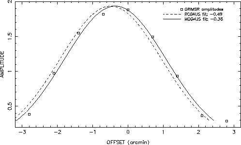
ORIMSR. The amplitude was measured at 9 positions which are summarized in Table 1 and fig. 1. These measurements are
analyzed by fitting a Gaussian using three different techniques. The three
methods are described in detail in the appendices. Here it is sufficient to
know that RCGAUS is the subroutine used by program CROSS. In
addition we use a cross-correlation fitting program (CCGAUS)
which provides a quick and dirty fit to position only, as well as a non-linear
least-squares algorithm (MQGAUS) based on the
Levenberg-Marquardt method (see "Numerical Recipes", Press et al. ,
p. 526) which also returns an estimate of the peak of the gaussian and
(optionally) an estimate of the full-width at half-power of the primary beam.
Table 1: Example pointing measurements of source ORIMSR
on March 14, 1991.
       Delta Elevation   Amplitude
       ---------------------------
	   -2.8            0.385
	   -2.1            0.972
	   -1.4            1.550
	   -0.7            1.818
	    0.0            1.883
	    0.7            1.493
	    1.4            0.930
	    2.1            0.363
	    2.8            0.285

Figure 1: Offset pointing measurements on ORIMSR (squares) and best fit Gaussian
from RCGAUS (dashed) and MQGAUS (solid).
Cross reports a position offset of -0.49 arcminutes and subroutine RCGAUS also returns an offset of -0.49 arcmin when called by a
local driver program. In contrast, CCGAUS and MQGAUS find an offset of -0.35 and -0.36 arcminutes
respectively (fig. 1). This discrepancy deserve further
examination.
Errors in the fitting routines RCGAUS, CCGAUS, and MQGAUS, can be quantified by
calling each routine with an exact offset Gaussian of the form

where A(x) is the amplitude at position x, xo is the
true offset, and FW is the full-width at half maximum of the pattern,
in this case 3.4 arcmin. The 3.4 arcmin pattern width is equivalent to 2.4
arcmin full-width at half-power of the individual antenna beams. That is, CROSS
measures the voltage pattern of the primary beam rather than the power
pattern.
We first consider a set of 9 measurements at a spacing of 0.7 arcmin with no
noise. This spacing is the default for POINT.COM. For each model offset
xo the difference of the fit offset from the true offset
delta(xo) = xfit - xo is calculated and shown in
Table 2.
Table 2: Errors fitting exact offset Gaussians with 9 by
0.7 arcmin sampling.
       xo   Error: delta(xo) = xfit - xo (arcmin)
    (arcmin)    RCGAUS    CCGAUS    MQGAUS
    --------------------------------------------
    -0.5       -0.20        0.02      0.00
    -0.1       -0.04        0.00      0.00
     0.0        0.00        0.00      0.00
     0.1        0.04        0.00      0.00
     0.2        0.08       -0.01      0.00
     0.5        0.20       -0.02      0.00
     1.0        0.47       -0.08      0.00
     1.5        1.02       -0.19      0.00
     2.0        0.80       -0.37      0.00
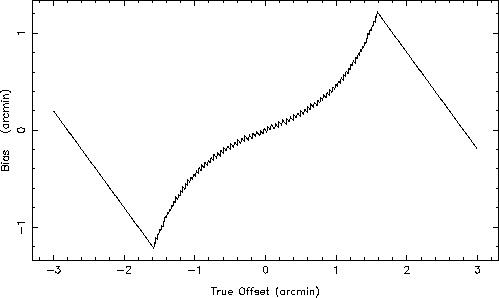
The results of fitting an exact offset Gaussian indicate that RCGAUS introduces a positive bias in the fit which increases in
magnitude with increasing offset. The error approaches 70% for offsets of 1.5
arcmin as shown in fig. 2. Even for small offsets, the error
is clearly biased in the direction of the offset. As expected, the magnitude of
the error is the same for negative or positive offsets. CCGAUS also introduces a bias, although with smaller magnitude
and in the opposite sense. The solution from MQGAUS,
however, is exact, as might be expected from a non-linear fitting routine.

Figure 2: Systematic bias in offset fitting
of true Gaussian with sampling of 9 by 0.7 arcmin.
The errors in RCGAUS and CCGAUS can be
decreased by increasing the number of steps or increasing the step size or both,
as shown in Table 3 for an offset of 0.5 arcmin. It is
clear, however, that cross-correlation methods fails in the fitting of exact
Gaussians with no noise. Next, we consider the addition of noise.
Table 3: Errors fitting 0.5 arcmin offset Gaussians.
   Number     size   Error: delta(xo) = xfit - xo (arcmin)
   of steps (arcmin)    RCGAUS    CCGAUS    MQGAUS
   ---------------------------------------------------
       9      0.7        0.20     -0.02      0.00
       9      0.9        0.04      0.00      0.00
       9      1.0        0.00      0.00      0.00
      11      0.7        0.06      0.00      0.00
      11      0.8        0.02      0.00      0.00
We next consider fitting an offset Gaussian with additive random noise described
by

where noise is normally distributed with zero mean and
unit variance, and SNR is the signal-to-noise ratio for each measurement of
amplitude. The average error of the fit is calculated from 400 trials and the
results are summarized in Table 4 for the case SNR =10.
Table 4:
Errors in fitting Gaussians plus noise with SNR=10 anr 9 by 0.7 arcmin sampling.
       xo   Error: delta(xo) = xfit - xo (arcmin)
    (arcmin)    RCGAUS      CCGAUS     MQGAUS
    --------------------------------------------
     -0.5       -0.18        0.02       0.00
     -0.1       -0.04        0.00       0.00
      0.0        0.00        0.00       0.00
      0.1        0.04       -0.01       0.00
      0.2        0.07       -0.01       0.00
      0.5        0.17       -0.03      -0.01
      1.0        0.48       -0.08       0.00
      1.5        1.03       -0.18       0.01
      2.0        0.80       -0.37       0.01
The errors in fitting Gaussians with additive noise are similar to the case with
no noise. Thus the conclusions are the same as before. Namely, that RCGAUS and CCGAUS yield biased results in
fitting for position offsets. A non-linear method is clearly superior in fitting
for position offset. This can be demonstrated by considering the extreme case of
fitting just 2 points with SNR =10, measured at the half-power separation of 2.4
arcminutes. The results in Table 5 show that MQGAUS finds a good solution for pointing errors as large as
1.5 arcmin.
Table 5: Errors in fitting Gaussians plus noise
with SNR=10 and 2 by 2.4 arcmin sampling.
       xo   Error: delta(xo) = xfit - xo (arcmin)
    (arcmin)    RCGAUS      CCGAUS     MQGAUS
    --------------------------------------------
      0.0        0.13        0.06       0.01
      0.1        0.91        0.43       0.00
      0.2        1.00        0.45       0.00
      0.5        0.70        0.27       0.02
      1.0        0.20       -0.04       0.02
      1.5       -0.30       -0.42       0.10
      2.0       -0.80       -0.87      -0.21
The net effect of the bias introduced by CROSS can be evaluated by analyzing the
pointing fitting for the B3 configuration (see BIMA
memo #2 "Hat Creek Interferometer Pointing Fitting", M. Wright,
3-Jan-1990). Assuming that the B3 data was obtained with sampling of 9 by 0.7
arcmin, the results shown in fig. 2 can then be applied to the
data to remove the bias. The results of pointing fitting before and after
correction for the bias is summarized in Table 6. The
pointing constants have changed slightly and the RMS deviations have been
reduced. In some cases, the RMS approaches that obtained by optical pointing.
In conclusion, it is clear that a large fraction of the dispersion in the radio
pointing is a result of systematic error introduced by subroutine RCGAUS. It is
strongly recommended that RCGAUS be replace by an improved method such as
MQGAUS.
Table 6: Analysis of B3 pointing data
Ant           Pointing constants 1--7 (arcmin)     RMS (arcsec)
---------------------------------------------------------------
Original data with bias:
1 APC    -29.59  0.47 -0.01 -1.59 -5.17  0.29 0.83     12
1 EPC     11.07  0.35  0.24 -0.25 -0.30  0.04 0.91     29
2 APC    -21.45  2.80  0.88 -3.62 -1.90  0.59 0.47     24
2 EPC     71.32  0.47  0.26 -0.31  0.12  0.18 0.92     16
3 APC     18.41  2.22  0.96 -0.13 -0.72  0.40 0.32     13
3 EPC      5.11 -0.42  1.39 -0.51 -0.18 -0.28 0.82     17

After correction for bias:
1 APC    -29.94  0.59 -0.17 -1.42 -4.63  0.25 0.55     08
1 EPC     11.04  0.40  0.40 -0.05 -0.20 -0.03 0.83     14
2 APC    -21.74  2.78  1.00 -3.72 -1.66  0.50 0.42     15
2 EPC     71.23  0.43  0.19 -0.31  0.24  0.17 0.94     10
3 APC     18.37  2.11  1.05 -0.13 -0.67  0.36 0.33     11
3 EPC      5.14 -0.44  1.08 -0.32 -0.04 -0.31 0.90     11
C------------------------------------------------------------C
SUBROUTINE RCGAUS(X,Y,NPTS,XCEN,THRESH,BADFIT,RATIO)
C CONVOLVES DATA ARRAY WITH 3.2' FWHM GAUSSIAN TO FIND
C POINTING OFFSET XCEN
C------------------------------------------------------------C
REAL X(*),Y(*)
ALPHA=-4.*ALOG(2.)/3.2**2
X0=X(1)
DELTA=(X(2)-X(1))/10.
HFIT=0.
10 SUM=0.
TWGT=0.
DO 20 I=1,NPTS
WGT=EXP(ALPHA*(X(I)-X0)**2)
TWGT=TWGT+WGT
20 SUM=SUM+Y(I)*WGT
FIT=SUM/TWGT
IF(X0 .EQ. X(1)) FFIT=FIT
IF (FIT.LE.HFIT) GO TO 30
HFIT=FIT
XCEN=X0
30 X0=X0+DELTA
IF (X0.LE.X(NPTS)) GO TO 10
BADFIT=0.
IF(HFIT/FFIT .LT. THRESH .AND. HFIT/FIT .LT. THRESH) BADFIT=-1.
RATIO=HFIT/FFIT
IF(RATIO .LT. HFIT/FIT) RATIO=HFIT/FIT
RETURN
END
SUBROUTINE CCGAUS (X,Y,NPTS,FWHM,XCEN,THRESH,BADFIT,RATIO)
C
C This subroutine is used to find the pointing offset of a gaussian beam
C given a set of 1-dimensional measurements.
C
C INPUTS:
C
C X(*) REAL*4 Array of offsets in arcminutes
C Y(*) REAL*4 Array of amplitude measurements
C NPTS INTEGER Number of measurements in X and Y
C FWHM REAL*4 Full-Width Half-Power of primary beam (2.4 arcmin?)
C THRESH REAL*4 Threshold for badfit calculation
C
C OUTPUTS:
C
C XCEN REAL*4 Offset in units of X
C BADFIT REAL*4 0.0 for good fit, -1.0 otherwise
C RATIO REAL*4 Used in calculation of BADFIT
C
integer npts, i
real x(*), y(*), xcen, thresh, badfit, ratio, x0, alpha,
& sum, fit, fit1, fit2, FWHM
alpha = -2.0*alog(2.0)/FWHM**2.0
badfit = 0.0
fit = 0.0
do x0 = x(1), x(npts), 0.01
sum = 0.0
do i = 1, npts
sum = sum + y(i)*exp(alpha*(x(i)-x0)**2.0)
end do
if (x0 .eq. x(1)) fit1 = sum
if (sum .gt. fit) then
fit = sum
xcen = x0
end if
end do
fit2 = sum
badfit = 0.0
if (fit/fit1.lt.thresh .AND. fit/fit2.lt.thresh) badfit = -1.0
ratio = min(fit/fit1,fit/fit2)
return
end
SUBROUTINE MQGAUS(X,Y,N,XCEN,PEAK,FWHM,CHISQ,BADFIT)
C
C This subroutine uses the non-linear Levenberg-Marquardt method
C (see "Numerical Recipes", W. H. Press et al., p. 526)
C to fit a Gaussian to a set of measurements. It returns the offset
C of the Gaussian, and can optionally fit for the peak and width of
C the Gaussian.
C
C INPUTS:
C
C X(*) REAL*4 Array of offset values (arc-minutes)
C Y(*) REAL*4 Array of measured amplitudes.
C N INTEGER Number of points in X and Y
C PEAK REAL*4 For PEAK > 0, will use as initial guess of maximum of
C Gaussian and return best fit value. For PEAK < 0 will
C use ABS(PEAK) in fit and hold constant.
C FWHM REAL*4 For FWHM > 0, will use as initial guess of width of
C Gaussian and return best fit value. For FWHM < 0 will
C use ABS(FWHM) in fit and hold constant.
C OUTPUTS:
C
C XCEN REAL*4 Best fit offset position in units of X
C PEAK REAL*4 For PEAK > 0 on input, best fit on output
C FWHM REAL*4 For FWHM > 0 on input, best fit on output
C CHISQ REAL*4 Chi-squared of fit
C BADFIT REAL*4 badfit = -1.0 if no convergence after 10 iterations
C
C HINTS:
C
C To find the offset for a given set of pointing measurements, call
C this subroutine with PEAK = ,
C and FWHM = -2.4. This just fits for offset and peak.
C
C
integer n, i, lista(3), mfit
real x(*), y(*), peak, xcen, fwhm,
& a(3), chisq1, chisq, alamda1, alamda,
& alpha(3,3), covar(3,3), fgauss
external fgauss
xcen = 0.0
badfit = 0.0
mfit = 1
lista (1) = 1
lista (2) = 0
lista (3) = 0
a(1) = 0.0
if (peak .ge. 0) then
mfit = mfit + 1
lista(mfit) = 2
a(2) = abs(peak)
else
a(2) = abs(peak)
end if
if (fwhm .ge. 0) then
mfit = mfit + 1
lista(mfit) = 3
a(3) = abs(fwhm)
else
a(3) = abs(fwhm)
end if
alamda = -1.0
alamda1 = 0.01
chisq1 = 1.0E10
do i = 1, 10
call mrqmin(x,y,n,a,3,lista,mfit,covar,
& alpha,3,chisq,fgauss,alamda)
if (abs(chisq1-chisq).lt.1.E-5) goto 20
if (alamda .gt. alamda1) goto 10
chisq1 = chisq
alamda1 = alamda
end do
10 badfit = -1.0
return
20 continue
alamda=0.0
call mrqmin(x,y,n,a,3,lista,mfit,covar,
& alpha,3,chisq,fgauss,alamda)
xcen = a(1)
peak = a(2)
fwhm = a(3)
return
end
SUBROUTINE MRQMIN(X,Y,NDATA,A,MA,LISTA,MFIT,
* COVAR,ALPHA,NCA,CHISQ,FUNCS,ALAMDA)
PARAMETER (MMAX=20)
DIMENSION X(*),Y(*),A(*),LISTA(*),
* COVAR(NCA,NCA),ALPHA(NCA,NCA),ATRY(MMAX),BETA(MMAX),DA(MMAX)
IF(ALAMDA.LT.0.)THEN
KK=MFIT+1
DO 12 J=1,MA
IHIT=0
DO 11 K=1,MFIT
IF(LISTA(K).EQ.J)IHIT=IHIT+1
11 CONTINUE
IF (IHIT.EQ.0) THEN
LISTA(KK)=J
KK=KK+1
ELSE IF (IHIT.GT.1) THEN
PAUSE 'Improper permutation in LISTA'
ENDIF
12 CONTINUE
IF (KK.NE.(MA+1)) PAUSE 'Improper permutation in LISTA'
ALAMDA=0.001
CALL MRQCOF(X,Y,NDATA,A,MA,LISTA,MFIT,ALPHA,BETA,NCA,CHISQ,F
*UNCS)
OCHISQ=CHISQ
DO 13 J=1,MA
ATRY(J)=A(J)
13 CONTINUE
ENDIF
DO 15 J=1,MFIT
DO 14 K=1,MFIT
COVAR(J,K)=ALPHA(J,K)
14 CONTINUE
COVAR(J,J)=ALPHA(J,J)*(1.+ALAMDA)
DA(J)=BETA(J)
15 CONTINUE
CALL GAUSSJ(COVAR,MFIT,NCA,DA,1,1)
IF(ALAMDA.EQ.0.)THEN
CALL COVSRT(COVAR,NCA,MA,LISTA,MFIT)
RETURN
ENDIF
DO 16 J=1,MFIT
ATRY(LISTA(J))=A(LISTA(J))+DA(J)
16 CONTINUE
CALL MRQCOF(X,Y,NDATA,ATRY,MA,LISTA,MFIT,COVAR,DA,NCA,CHISQ,FU
*NCS)
IF(CHISQ.LT.OCHISQ)THEN
ALAMDA=0.1*ALAMDA
OCHISQ=CHISQ
DO 18 J=1,MFIT
DO 17 K=1,MFIT
ALPHA(J,K)=COVAR(J,K)
17 CONTINUE
BETA(J)=DA(J)
A(LISTA(J))=ATRY(LISTA(J))
18 CONTINUE
ELSE
ALAMDA=10.*ALAMDA
CHISQ=OCHISQ
ENDIF
RETURN
END
SUBROUTINE FGAUSS(X,A,Y,DYDA,NA)
DIMENSION A(NA),DYDA(NA)
Y=0.
DO 11 I=1,NA-1,3
ARG=(X-A(I))/A(I+2)
EX=EXP(-2.0*ALOG(2.0)*ARG**2)
FAC=2.0*ALOG(2.0)*A(I+1)*EX*2.*ARG
Y=Y+A(I+1)*EX
DYDA(I)=FAC/A(I+2)
DYDA(I+1)=EX
DYDA(I+2)=FAC*ARG/A(I+2)
11 CONTINUE
RETURN
END
SUBROUTINE COVSRT(COVAR,NCVM,MA,LISTA,MFIT)
DIMENSION COVAR(NCVM,NCVM),LISTA(*)
DO 12 J=1,MA-1
DO 11 I=J+1,MA
COVAR(I,J)=0.
11 CONTINUE
12 CONTINUE
DO 14 I=1,MFIT-1
DO 13 J=I+1,MFIT
IF(LISTA(J).GT.LISTA(I)) THEN
COVAR(LISTA(J),LISTA(I))=COVAR(I,J)
ELSE
COVAR(LISTA(I),LISTA(J))=COVAR(I,J)
ENDIF
13 CONTINUE
14 CONTINUE
SWAP=COVAR(1,1)
DO 15 J=1,MA
COVAR(1,J)=COVAR(J,J)
COVAR(J,J)=0.
15 CONTINUE
COVAR(LISTA(1),LISTA(1))=SWAP
DO 16 J=2,MFIT
COVAR(LISTA(J),LISTA(J))=COVAR(1,J)
16 CONTINUE
DO 18 J=2,MA
DO 17 I=1,J-1
COVAR(I,J)=COVAR(J,I)
17 CONTINUE
18 CONTINUE
RETURN
END
SUBROUTINE MRQCOF(X,Y,NDATA,A,MA,LISTA,MFIT,ALPHA,BETA,NALP,
* CHISQ,FUNCS)
PARAMETER (MMAX=20)
DIMENSION X(*),Y(*),ALPHA(NALP,NALP),BETA(MA),
* DYDA(MMAX),LISTA(*),A(MA)
DO 12 J=1,MFIT
DO 11 K=1,J
ALPHA(J,K)=0.
11 CONTINUE
BETA(J)=0.
12 CONTINUE
CHISQ=0.
DO 15 I=1,NDATA
CALL FUNCS(X(I),A,YMOD,DYDA,MA)
DY=Y(I)-YMOD
DO 14 J=1,MFIT
WT=DYDA(LISTA(J))
DO 13 K=1,J
ALPHA(J,K)=ALPHA(J,K)+WT*DYDA(LISTA(K))
13 CONTINUE
BETA(J)=BETA(J)+DY*WT
14 CONTINUE
CHISQ=CHISQ+DY*DY
15 CONTINUE
DO 17 J=2,MFIT
DO 16 K=1,J-1
ALPHA(K,J)=ALPHA(J,K)
16 CONTINUE
17 CONTINUE
RETURN
END
SUBROUTINE GAUSSJ(A,N,NP,B,M,MP)
PARAMETER (NMAX=50)
DIMENSION A(NP,NP),B(NP,MP),IPIV(NMAX),INDXR(NMAX),INDXC(NMAX)
DO 11 J=1,N
IPIV(J)=0
11 CONTINUE
DO 22 I=1,N
BIG=0.
DO 13 J=1,N
IF(IPIV(J).NE.1)THEN
DO 12 K=1,N
IF (IPIV(K).EQ.0) THEN
IF (ABS(A(J,K)).GE.BIG)THEN
BIG=ABS(A(J,K))
IROW=J
ICOL=K
ENDIF
ELSE IF (IPIV(K).GT.1) THEN
PAUSE 'Singular matrix'
ENDIF
12 CONTINUE
ENDIF
13 CONTINUE
IPIV(ICOL)=IPIV(ICOL)+1
IF (IROW.NE.ICOL) THEN
DO 14 L=1,N
DUM=A(IROW,L)
A(IROW,L)=A(ICOL,L)
A(ICOL,L)=DUM
14 CONTINUE
DO 15 L=1,M
DUM=B(IROW,L)
B(IROW,L)=B(ICOL,L)
B(ICOL,L)=DUM
15 CONTINUE
ENDIF
INDXR(I)=IROW
INDXC(I)=ICOL
IF (A(ICOL,ICOL).EQ.0.) PAUSE 'Singular matrix.'
PIVINV=1./A(ICOL,ICOL)
A(ICOL,ICOL)=1.
DO 16 L=1,N
A(ICOL,L)=A(ICOL,L)*PIVINV
16 CONTINUE
DO 17 L=1,M
B(ICOL,L)=B(ICOL,L)*PIVINV
17 CONTINUE
DO 21 LL=1,N
IF(LL.NE.ICOL)THEN
DUM=A(LL,ICOL)
A(LL,ICOL)=0.
DO 18 L=1,N
A(LL,L)=A(LL,L)-A(ICOL,L)*DUM
18 CONTINUE
DO 19 L=1,M
B(LL,L)=B(LL,L)-B(ICOL,L)*DUM
19 CONTINUE
ENDIF
21 CONTINUE
22 CONTINUE
DO 24 L=N,1,-1
IF(INDXR(L).NE.INDXC(L))THEN
DO 23 K=1,N
DUM=A(K,INDXR(L))
A(K,INDXR(L))=A(K,INDXC(L))
A(K,INDXC(L))=DUM
23 CONTINUE
ENDIF
24 CONTINUE
RETURN
END


