LineFit (Part 2)
Here we have a classic example of fitting a line two ways: take two
observables, X and Y. Normally we assume the error is in Y and X
is an independant variable with no error. But we add a few twists:
- X and Y are really LOG(X) and LOG(Y), but ignoring issues of errors in linear of log space
- there is an error in X (well, LOG(X)), as well
- we also fit LOG(Y/X) vs. LOG(X), to see how much LOG(Y/X) is biased
There are two scripts: linefit2.csh,
which is being called by linefit2a.csh to run a lot
of them, assemble some basic numbers in a table, and then plot these up
with tabhist.
Although we only use the OLS(Y/X) method in
linreg, you could also play with bisector
or other fits to get a less biased fit. This example is just to show you the
amount of the bias for given errors in X and Y.
Here's the example: 1000 random samples of a fit with slope 0.55 and intercept 4.0.
There are 90 points between 7 and 11.5.
The expected slope in LOG(Y/X) should be 0.55-1 = -0.45. Errors of 0.5 in both X
and Y have been added.
  linefit2a.csh n=1000 sx=0.5 sy=0.5 > sx_0.5b.tab
	(takes about 12" to run)

  tabhist sx_0.5b.tab 2 xmin=0.35 xmax=0.75 xcoord=0.55 yapp=linefit2a.gif/gif
  tabhist sx_0.5b.tab 3 xmin=0.35 xmax=0.75 xcoord=0.55 yapp=linefit2b.gif/gif
  tabhist sx_0.5b.tab 4 xmin=-0.65 xmax=-0.25 xcoord=-0.45 yapp=linefit2c.gif/gif
The 3 plots below show these correlations, the vertical line in the middle
is the correct answer if there was no error in X.
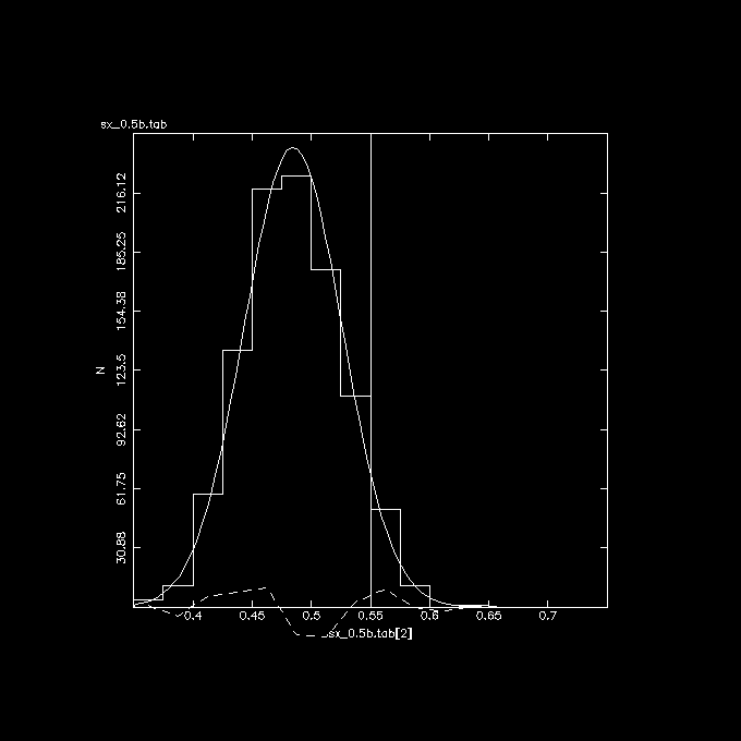 Y vs. X (observed) , indeed slope is flattened from the expected 0.55
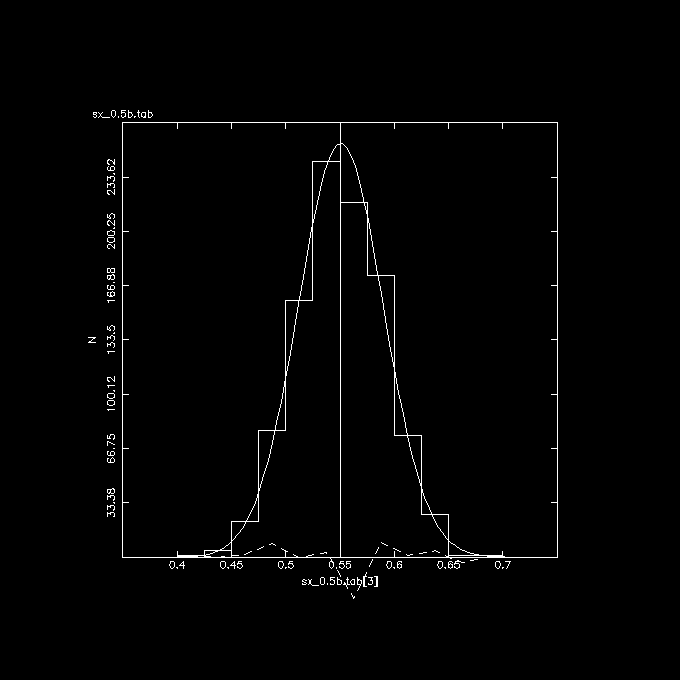 Y vs. X (no errors), indeed nicely centered at the expected 0.55
 Y/X vs. X (observed), again shifted from the expected -0.45 value, by the
same amount as Y vs. X (observed).
Y/X vs. X (observed), again shifted from the expected -0.45 value, by the
same amount as Y vs. X (observed).
Another wrapper on top of linefit2a.csh was written to see how this
error depended on the input error in X and Y. Turns out that it roughly
grows quadratically:
