First we describe a simple example how to run partiview with a supplied sample
dataset. Then we describe the different windows that partiview is made up of, and
the different commands and keystrokes it listens to.
Start the program using one of the sample "speck" files in the
data directory:
       % cd partiview/data
       % ./hipbright
or
       % partiview hipbright
and this should come up with a display familiar to most of us who
watch the skies. You should probably enlarge the
window a bit. Mine comes up in roughly a 300 by 300 display window,
which may be a bit small (certainly on my screen :-)
(Hint: the .partiviewrc file may contain commands like
eval winsize 600 400.)
Hit the TAB key to bring focus to the (one line) command window inbetween the log screen (top) and viewing screen (bottom). Type the commands
        fov 50                          (field of view 50 degrees)
        jump 0 0 0 80 70 60             (put yourself in the origin
                                        and look at euler angles
                                        RxRyRz (80,70,60)
and it should give another nice comfy view :-) If you ever get lost,
and this is not hard, use
the jump command to go back to a known position and/or viewing
angle.
Note that spatial units for this dataset are parsecs, though angular units are degrees for any data in partiview.
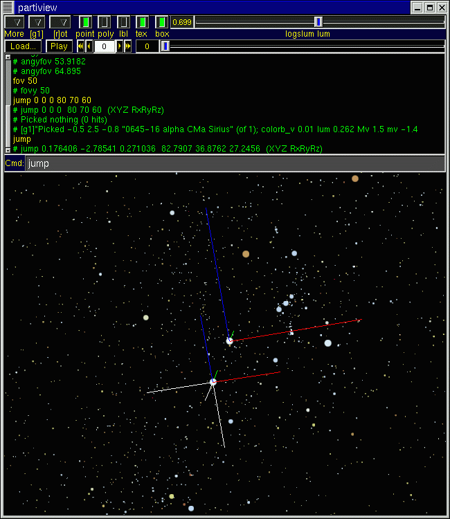
Now play with the display, use the 't', 'r', 'f' and 'o' keys (keys are case sensitive) in the viewing window and use the left and mouse buttons down to (carefully) move around a bit, and make yourself comfortable with moving around. Using the 't' button you get some idea of the distance of the stars by moving back and forth a little (the parallax trick). In fact, if you 't' around a little bit, you may see a green line flashing through the display. This is one of the RGB (xyz) axes attached to the (0,0,0) [our sun] position. You should see Procyon and Sirius exhibit pretty large parallaxes, but Orion is pretty steady since it is several hundred parsecs away. If you move the right mouse button you will zoom in/out and should see our Sun flash by with the red-green-blue axes.
The RGB axes represent the XYZ axes in a (right-handed) cartesian system. For the Hipparcos data the X (red) axis points to RA=0h, Y (green) axis to RA=6h, both in the equatorial plane, and the Z (blue) axis points to the equatorial north pole.
Try and use the middle mouse button (or the 'p' key) to click on Sirius or Procyon, and see if you can get it to view its properties. Now use the 'P' key to switch center to rotation to that star. Sirius is probably a good choice. Move around a bit, and try and get the sun and orion in the same view :-)
[NOTE: these Hipparcos data do not have reliably distance above 100-200 pc, so Orion's individual distances are probably uncertain to 30%]
A little bit on the types of motion, and what the mouse buttons do
              |     left            middle          right
              |     Button-1        Button-2        Button-3         Shift Button-1
------------------------------------------------------------------------------------
f (fly)       |     fly             'pick'          zoom
o (orbit)     |     orbit           'pick'          zoom
r (rotate)    |     rotate X/Y      'pick'          rotate Z            translate
t (translate) |     translate       'pick'          zoom
The point of origin for rotations can be changed with the 'P' button. First you can try and pick ('p' or Button-2) a point, and if found, hit 'P' to make this point the new rotation center default.
red   = X axis
green = Y axis
blue  = Z axis
To choose an arbitrary center of rotation, use the center command.
The top row contains some shortcuts to some frequently used commands. From left to right, it should show the following buttons:
Offers some mode switches as toggles: inertia
for continues spin or motion,
and an H-R Diagram to invoke a separate H-R diagram window
for datasets that support stellar evolution.
Pulldown g1, g2, ... (or whichever group)
is the currently selected group. See object command
to make aliases which group is defined to what object. If multiple
groups are defined, the next row below this contains a list of all
the groups, and their aliases, so you can toggle them to be displayed.
Pulldown to select fly/orbit/rot/tran, which can also be activate by pressing the f/o/r/t keys inside the viewing window.
Toggle to turn the points on/off. See also the points command.
Toggle to turn polygons on/off. See also the polygon command.
Toggle to turn labels on/off. See also the label command.
Toggle to turn textures on/off. See also the texture command.
Toggle to turn boxes on/off. See also the boxes command.
The current displayed value of the logslum lum slider (see next)
Slider controlling the logarithm of the datavar variable
selected as luminosity (with the lum command).
When more than one group has been activated (groups of particles or objects can have their own display properties, and be turned on and off at will), a new Group Row will appear as the 2nd row.
Left-clicking (button 1) on a button toggles the display of that group; right-clicking (button 3) enables display of the group, and also selects it as the current group for GUI controls and text commands.
For time-dependent data, the third and fourth row from the top control the currently displayed data-time. This time-control bar is only visible when the object has a nonzero time range.
Shows the current time (or offset from the tripmeter).
The absolute time is the sum of the T and + fields.
Both are editable.
See also the step control command.
Press to mark a reference point in time. The T field becomes zero, and the + field (below) is set to current time. As time passes, T shows the offset from this reference time.
Press to return to reference time (sets T to 0).
Current last time where tripmeter was set. You can reset to
the first frame with the command step 0
Drag to adjust the current time. Sensitivity depends on the speed setting; dragging by one dial-width corresponds to 0.1 wall-clock second of animation, i.e. 0.1 * speed in data time units.
Step time backwards or forwards by 0.1 * speed data time units.
See also the < and > keyboard shortcuts.
toggle movie move forwards in time
Toggle animating backwards or forwards in time, by
1 * speed data time units per real-time second.
See also the {, ~, and } keyboard shortcuts.
(Logarithmic) value denoting speed of animation.
See also the speed control command.
The fifth (or 4th or 3rd, depending if Group and/or Time rows are present) row from the top controls loading and playing sequences of moving through space.
Brings up a filebrowser to load a .wf path file. This is a file with on each
line 7 numbers: xyz location, RxRyRz viewing direction, and FOV (field of view).
The rdata command loads such path files too.
Play the viewpoint along the currently loaded path,
as the play command does.
Right-click for a menu of play-speed options.
Step through camera-path frames.
See also frame control command.
Slides through camera path, and displays current frame.
The third window from the top contains a logfile of past commands and responses to them, and can be resized by dragging the bar between command window and viewing window. The Logfile window also has a scroll bar on the left. You can direct the mouse to any previous command, and it will show up in the command window. Using the arrow keys this command can then be edited.
The Command window is a single line entry window, in which Control
Commands can be given. Their responses appear in the Logfile
window and on the originating console. (unlike Data Commands,
which show no feedback). You can still give Data Commands in
this window by prefixing them with the add command.
The Up- and Down-arrow keys (not those on the keypad) scroll through
previous commands, and can be edited using the arrow keys and a subset
of the emacs control characters.
The (OpenGL) Viewing window is where all the action occurs. Typically this is where you give single keystroke commands and/or move the mouse for an interactive view of the data. It can be resized two ways: either by resizing the master window, or by picking up the separator between Viewing window and Command window above.
Setting up a small animation in for example Starlab can be done quite simply as follows: (see also the primbim16.mk makefile to create a standard one):
  % makeplummer -i -n 20 | makemass -l 0.5 -u 10.0 | scale -s | kira -d 2 -D x10 > run1
  % partiview run1.cf
  % cat run1.cf

  kira run1
  eval every
  eval lum mass 0 0.01
  eval psize 100
  eval cment 1  1 .7 .3
  eval color clump exact
Alternatively, if you had started up partiview without any arguments, the following Control Command (see below) would have done the same
read run1.cf
The 's' key within the viewing window toggles stereo viewing. By default each object is split in a blue and a red part, that should be viewed with a pair of red(left)/blue(right) glasses. Red/green glasses will probably work too. Crosseyed viewing is also available if selected by stereo cross. See stereo and focallen in the View Commands section.
In the data directory, run
partiview hip.cfOne of the data fields for these stars is the B-V color,
colorb_v,
abbreviatable to just color. Look at just the bluest stars: try
thresh color < -.1Back off to a large distance (drag with right mouse button, and drag the
logslum lum slider to brighten)
and look at the distribution of these blue stars. The
Orion spiral-arm spur, extending generally along the +Y (green)
axis, has lots of them. Now look at more reddish stars,
those with .5 <= B-V <= 1.5, with:
thresh color .5 1.5These are much more uniformly distributed in the galactic plane. Return to seeing all stars, with:
see allor re-view the threshold-selected subset (reddish stars) with
see threshor its complement with
see -thresh